Load Data
# Load the merged mass spectrometry data and compound scaffold group data
ms_data_merged <- readRDS("ms_data_merged.Rds")
cpds_scaffold_group <- readRDS("cpds_lscaffold_group.Rds")
Data Preparation
Prepare Compound Data
# Generate a data frame by modifying compound ID names
x <- data.frame(
  `Compound ID` = ms_data_merged %>% names() %>%
    str_remove(pattern = "_THP1*") %>%
    str_remove(pattern = "_3v[1-2]*") %>%
    str_remove(pattern = "_002") %>%
    str_remove(pattern = ".[0-9]nd|.[0-9]rd|[4-9]th"),
  file = ms_data_merged %>% names(),
  check.names = FALSE
) %>%
  full_join(cpds_scaffold_group)
## Joining with `by = join_by(`Compound ID`)`
# Create a summary data frame for group counts
gg_data <- cpds_scaffold_group %>%
  group_by(Group) %>%
  mutate(count = n()) %>%
  select(-2) %>%
  distinct() %>%
  na.omit()
Calculate Frequency Data for Plotting
# Create frequency data frame and calculate frequencies
y <- data.frame(
  `Compound ID` = ms_data_merged %>% names() %>%
    str_remove(pattern = "_THP1*") %>%
    str_remove(pattern = "_3v[1-2]*") %>%
    str_remove(pattern = "_002") %>%
    str_remove(pattern = ".[0-9]nd|.[0-9]rd|[4-9]th"),
  file = ms_data_merged %>% names(),
  check.names = FALSE
) %>%
  left_join(cpds_scaffold_group) %>%
  na.omit() %>%
  filter(!duplicated(`Compound ID`)) %>%
  pull(Group) %>%
  table() %>%
  as.data.frame() %>%
  set_names(c("Group", "MS_counts"))
## Joining with `by = join_by(`Compound ID`)`
# Merge data for plotting with frequency
gg_part_data <- gg_data %>%
  left_join(y) %>%
  na.omit() %>%
  mutate(Freq = (MS_counts / count) %>% format(digits = 1))
## Joining with `by = join_by(Group)`
Plotting
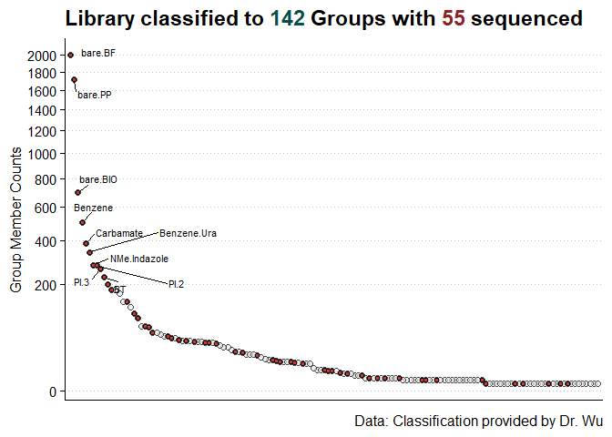
Plot 1: Group Member Counts
# Plot with group member counts and additional data labels
ggplot(gg_data, aes(x = reorder(Group, -count), y = count)) +
  geom_point(shape = 21, fill = "gray90", alpha = 0.7, size = 2, show.legend = FALSE) +
  scale_y_continuous(transform = "sqrt", name = "Group Member Counts", n.breaks = 15) +
  scale_x_discrete(name = NULL, expand = expansion(c(0.01, 0.01))) +
  ggthemes::theme_clean(base_size = 15) +
  theme(
    axis.text.x = element_blank(),
    axis.ticks.x = element_blank(),
    plot.title = element_markdown(),
    plot.background = element_rect(color = "white", fill = "white")
  ) +
  ggrepel::geom_text_repel(data = gg_data %>% arrange(-count) %>% head(10),
                           aes(label = Group),
                           max.overlaps = 20,
                           size = 3,
                           box.padding = 0.5) +
  labs(
    caption = "Data: Classification provided by Dr. Wu",
    title = paste0("Library classified to <span style='color:#084d49'>", nrow(gg_data),
                   "</span> Groups with <span style='color:brown4'>", nrow(gg_part_data), "</span> sequenced")
  ) +
  geom_point(data = gg_part_data, fill = "brown3", shape = 21)

# Save plot to file
# ggsave("group_plot.png", width = 8, height = 5)
Export Data to Excel
# Export frequency data to Excel
gg_data %>%
  left_join(y) %>%
  mutate(Freq = (MS_counts / count) %>% format(digits = 1)) %>%
  select(-2) %>%
  writexl::write_xlsx("freq.xlsx")
## Joining with `by = join_by(Group)`