简单记录boxplot可视化作图

library(tidyverse)
library(pheatmap)
library(RColorBrewer)
library(ggrepel)
library(multcompView)
library(ggpubr)
library(cowplot)
fpkm <- readxl::read_xlsx("hypophysoma.s180.FPKM.xlsx") %>% as.data.frame()
rownames(fpkm) <- fpkm$...1
fpkm <- fpkm %>% select(-"...1")
metadata <- read.table("SampleInfo_S180_order.txt", header = T, sep = "\t", quote = "")
head(metadata)
gene_ly6a <- read.table("Ly6 gene set.txt",  header = F, sep = "\t", quote = "")

pdf(file = "plot.pdf", width = 20, height = 10)
for (gene in cell_marker[cell_marker %in%  rownames(fpkm)]) {
  data <- fpkm[gene, ] %>% t() %>% as.data.frame()
  plot.data <- data %>% rownames_to_column() %>% left_join(metadata, by = c("rowname" = "SampleID"))

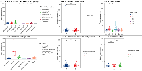
(p1 <- ggplot(data = plot.data, aes(x = WHO2017tumortype, y = get(gene), color = WHO2017tumortype)) +
  geom_boxplot(outlier.alpha = 0, show.legend = F) +
  geom_jitter(width = 0.2) +
  ggsci::scale_color_lancet() +
  ggthemes::theme_base() +
  labs(title = paste0(gene, " WHO2017tumortype Subgroups")) + 
  ylab("Gene expressions") +
  theme(axis.text.x = element_text(angle = 45, hjust = 1, vjust = 1), axis.title.x = element_blank())  +
  stat_compare_means(label = "p.signif", method = "t.test", ref.group = ".all.", hide.ns = T, show.legend = F))

(p2 <- ggplot(data = plot.data, aes(x = Subgoups, y = get(gene), color = Subgoups)) +
    geom_boxplot(outlier.alpha = 0, show.legend = F) +
    geom_jitter(width = 0.2) +
    ggsci::scale_color_lancet() +
    ggthemes::theme_base() +
    labs(title = paste0(gene, " Subgroups")) + 
    ylab("Gene expressions") +
    theme(axis.title.x = element_blank())  +
    stat_compare_means(label = "p.signif", method = "t.test", ref.group = ".all.", hide.ns = T, show.legend = F))

(p3 <- ggplot(data = plot.data, aes(x = Secretion, y = get(gene), color = Secretion)) +
  geom_boxplot(outlier.alpha = 0, show.legend = F) +
  geom_jitter(width = 0.2) +
  ggsci::scale_color_lancet() +
  ggthemes::theme_base() +
  labs(title = paste0(gene, " Secretion Subgroups")) + 
  ylab("Gene expressions") +
  theme(axis.text.x = element_text(angle = 45, hjust = 1, vjust = 1), axis.title.x = element_blank())+
  stat_compare_means(label = "p.signif", ref.group = ".all.", hide.ns = T, show.legend = F))

(p4 <-ggplot(data = plot.data, aes(x = Gender, y = get(gene), color = Gender)) +
  geom_boxplot(outlier.alpha = 0, show.legend = F) +
  geom_jitter(width = 0.2) +
  ggsci::scale_color_lancet() +
  ggthemes::theme_base() +
  labs(title = paste0(gene, " Gender Subgroups")) + 
  ylab("Gene expressions") +
  theme(axis.title.x = element_blank()) +
  ggsignif::geom_signif(comparisons = list(c("F", "M")), color ="black", map_signif_level = TRUE))

(p5 <-ggplot(data = plot.data, aes(x = CavernousInvasion, y = get(gene), color = CavernousInvasion)) +
  geom_boxplot(outlier.alpha = 0, show.legend = F) +
  geom_jitter(width = 0.2) +
  ggsci::scale_color_lancet() +
  ggthemes::theme_base() +
  labs(title = paste0(gene, " CavernousInvasion Subgroups")) + 
  ylab("Gene expressions") +
  theme(axis.title.x = element_blank()) +
  ggsignif::geom_signif(comparisons = list(c("N", "Y")), color ="black", map_signif_level = TRUE))

plot.data$TumorSizeClass <- ifelse(plot.data$TumorSizeMax >=3, ">= 3", ifelse(plot.data$TumorSizeMax < 1, "<1", "1 - 3"))
(p6 <-ggplot(data = plot.data, aes(x = TumorSizeClass, y = get(gene), color = TumorSizeClass)) +
  geom_boxplot(outlier.alpha = 0, show.legend = F) +
  geom_jitter(width = 0.2) +
  ggsci::scale_color_lancet() +
  ggthemes::theme_base() +
  labs(title = paste0(gene, " TumorSizeMax")) + 
  ylab("Gene expressions") +
  theme(axis.title.x = element_blank()) +
  ggsignif::geom_signif(comparisons = list(c(">= 3", "<1"), c(">= 3", "1 - 3"), c("1 - 3", "<1")), 
                        color ="black",y_position = c(0.85*max(plot.data[,(gene)]), 
                                                      0.9*max(plot.data[,(gene)]),
                                                      0.95*max(plot.data[,(gene)])), 
                        map_signif_level = TRUE))
p <- plot_grid(p1, p4, p2, p3, p5, p6, align = "v", ncol = 3, labels = "AUTO", rel_widths = c(1.3, 1,1, 1.3,1,1))
print(p)
}
dev.off()

ggsave("stem_marker2_plot.png", width = 20, height = 10)